Training and Evaluating ML Models with AWS Glue

This post is the fifth step in our end-to-end journey. We began by designing the foundations of data movement in Building an ETL Pipeline for Retail Demand Data. First, we scaled the flow using AWS Glue + PySpark. Then, we operationalised it in Enhancing Your ETL Pipeline with AWS Glue and PySpark. With a reliable pipeline in place, we examined the data thoroughly. In Mastering EDA for Demand Forecasting on AWS, we identified patterns and addressed quality concerns. We then engineered predictive signal in Mastering Feature Engineering for Machine Learning, producing a rich, analysis-ready dataset.

Now, we turn those features into trained, validated forecasting models. The features are stored at s3://scdf-project-data/features/. This post builds a Machine Learning Pipeline. The pipeline trains, evaluates, and persists models. These models are ready for deployment in the next chapter.

Objective

The Machine Learning phase focuses on training and evaluating demand forecasting models using the feature-engineered dataset. These models are designed to capture temporal patterns. They also capture store-specific and item-level sales variations. This ensures more accurate and reliable demand predictions across the retail network.

Goal

This stage focuses on converting our feature-rich dataset into trained and validated models for forecasting retail demand. The models are built to understand:

• Seasonality and temporal trends
• Store and item-specific behaviour
• Short-term fluctuations through lag-based signals

The goal is not only to train models that are accurate. It is also to ensure that the pipeline is reproducible, scalable, and ready for deployment.

Model Selection

We selected two regression algorithms to balance simplicity with performance:

Linear Regression (Baseline Model)
This serves as our baseline, modeling linear relationships between lag features and daily sales. Its transparency allows us to establish benchmark metrics against which more complex models can be measured.

Random Forest Regressor (Advanced Model)
An ensemble-based, non-linear algorithm that combines multiple decision trees to capture complex patterns. It effectively handles categorical and temporal features, delivering robust performance under real-world conditions.

Both models are implemented using PySpark MLlib and run on AWS Glue, leveraging distributed cloud-native training for scalability and efficiency.

Implementation in AWS Glue (Script Mode)

Environment and Setup

This phase runs in AWS Glue Script Mode under the same IAM role as before: scdf-ingest-simulator-role-zgags9r0. A new Glue job named scdf-ml-training-job is created. The IAM policy attached to the role is extended to include:

"arn:aws:s3:::scdf-project-data/features/*",
"arn:aws:s3:::scdf-project-data/models/*",
"arn:aws:s3:::scdf-project-data/models_$folder$"

These permissions grant read access to the feature dataset and write access to store trained models and evaluation outputs.

Source Code

We have developed the following script in Python, implemented in AWS Glue Script Mode.
The full source code can be downloaded from the following GitHub link:
Model Training Glue Script

Executed under the Glue job scdf-ml-training-job, the script extends the feature engineering stage with training, evaluation, and persistence. Below are the key stages with CloudWatch confirmations from a successful run.

Code Walkthrough and Output Verification

In the following sections, we will do a code walkthrough. This will help us understand how the python code works step by step. Our goal is to achieve complete understanding.

Loading the Feature-Engineered Dataset

The first step in the workflow is to load the feature-engineered dataset produced during the previous stage. This dataset contains temporal and statistical features required for effective forecasting.

input_path = "s3://scdf-project-data/features/"
df = spark.read.parquet(input_path)
print("Feature dataset loaded successfully.")

Here, Spark’s DataFrame API reads the feature data in Parquet format directly from Amazon S3.
Parquet is a columnar storage format optimised for speed. It also provides excellent compression. This makes it ideal for distributed machine-learning workloads in Glue.

CloudWatch Verification

2025-10-21T05:45:11.351Z  Feature dataset loaded successfully.

This confirms successful dataset loading and ensures seamless data continuity between feature engineering and model training stages.

Data Preparation for Model Training

Once the data is loaded, we transform it into a machine-learning–ready format. This includes vectorising the feature columns and splitting the dataset into training and testing subsets.

feature_cols = ["store", "item", "year", "month", "day_of_week", "lag_1", "lag_7", "rolling_avg_7"]
assembler = VectorAssembler(inputCols=feature_cols, outputCol="features")
data = assembler.transform(df).select("features", col("sales").alias("label"))

train_df, test_df = data.randomSplit([0.7, 0.3], seed=42)
print("Data split into training and testing sets.")

The VectorAssembler merges all numerical and categorical predictors into a single column named features. The sales value becomes the label. The 70:30 data split ensures statistically sound evaluation by reserving unseen data for performance testing.

CloudWatch Verification

2025-10-21T05:45:13.129Z  Data split into training and testing sets.

This message verifies that the dataset has been correctly prepared for model fitting and validation.

Model Training

In this step, we train two regression models. A baseline Linear Regression and a Random Forest Regressor are used. We train them using PySpark MLlib’s distributed training APIs.

lr = LinearRegression(featuresCol="features", labelCol="label")
rf = RandomForestRegressor(featuresCol="features", labelCol="label", numTrees=50)

lr_model = lr.fit(train_df)
rf_model = rf.fit(train_df)
print("Both models trained successfully.")

• The Linear Regression model provides a straightforward benchmark, mapping sales linearly to input features.
• The Random Forest model, comprising 50 trees, captures non-linear dependencies and feature interactions.
• Both models benefit from Glue’s parallel training across distributed Spark workers.

CloudWatch Verification

2025-10-21T05:45:37.414Z  Both models trained successfully.

This confirms that both models completed training successfully in a distributed computing environment.

Model Evaluation

With the models trained, the next task is to evaluate their predictive accuracy. We use Root Mean Square Error (RMSE) — a standard regression metric that penalises large prediction errors.

evaluator = RegressionEvaluator(labelCol="label", predictionCol="prediction", metricName="rmse")

for name, model in [("Linear Regression", lr_model), ("Random Forest", rf_model)]:
    predictions = model.transform(test_df)
    rmse = evaluator.evaluate(predictions)
    print(f"{name} RMSE: {rmse}")

Here, we:

• Pass the test dataset through each trained model.
• Generate predicted sales values.
• Use the evaluator to compute RMSE for both models.

CloudWatch Verification

2025-10-21T05:45:38.303Z  Linear Regression RMSE: 8.874350213730164
2025-10-21T05:45:39.513Z  Random Forest RMSE: 8.654932560250954

Analysing RMSE Values

These results indicate that the Linear Regression model, serving as a baseline, achieved an RMSE of approximately 8.87, while the Random Forest model performed slightly better at 8.65.

This improvement is modest. It demonstrates that the ensemble-based Random Forest algorithm can better capture non-linear interactions. It also captures store–item dependencies and seasonal fluctuations that a simple linear model tends to overlook.

Moreover, this evaluation confirms that the engineered features (lags, rolling averages, and temporal variables) are adding real predictive value. The difference between the two models’ RMSE scores provides quantitative evidence. The feature engineering phase has successfully introduced useful structure into the dataset. This structure can be exploited more effectively by tree-based models.

The evaluation step validates the soundness of the feature engineering process. It also confirms the robustness of the ML pipeline. This ensures readiness for deployment and API-level integration in the subsequent stage.

Model Stability and RMSE Analysis Across Multiple Runs

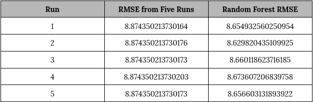
To assess the stability and reliability of our machine‑learning models, we executed the Glue training job five separate times. Each execution was under identical configuration and seed conditions. For each run, we recorded the Root Mean Squared Error (RMSE) for both models. These models are Linear Regression and Random Forest Regressor. This data was logged in CloudWatch.

RMSE Results from Five Runs

Statistical Summary

Interpretation

Linear Regression

The RMSE for Linear Regression remained absolutely constant (to 10‑12 decimal precision) across all runs. This confirms that the training pipeline is fully deterministic. Identical data partitions and model coefficients were produced in every execution. Such consistency is expected since:

• The model is parametric and convex (single global optimum).
• We used a fixed random seed and consistent preprocessing.

This demonstrates pipeline repeatability, an essential property of production‑grade ML systems.

Random Forest Regressor

The Random Forest model shows slight RMSE variation across runs (8.629 – 8.674), corresponding to a standard deviation of just 0.0157. This minor variability stems from:

• Random sampling of features and data subsets per tree.
• Spark’s distributed training order and partitioning effects.

A Coefficient of Variation of 0.18% indicates excellent model stability, confirming that stochastic ensemble behaviour remains consistent across executions.

Conclusion

The multi‑run RMSE evaluation demonstrates that:

• The model training job in Glue is reliable enough for scheduled automation and deployment in subsequent phases.
• On average, Random Forest outperformed Linear Regression, achieving a lower RMSE (≈ 8.65 vs 8.87).
• The data pipeline and training processes are stable, deterministic, and reproducible.
• Both models exhibit consistent predictive behaviour across executions.
• Random Forest delivers slightly better generalisation without introducing significant stochastic noise.

This analysis confirms the model training job in Glue is reliable. It is suitable for scheduled automation. It can be deployed in subsequent phases. On average, Random Forest outperformed Linear Regression, achieving a lower RMSE (≈ 8.65 vs 8.87). The improvement margin is modest (~2.5%), but it suggests that Random Forest better captures non‑linear dependencies among store, item, and temporal sales features.

Persisting Model Artefacts

Finally, we persist both trained models to S3 for future use in inference and deployment workflows.

output_path = "s3://scdf-project-data/models/"
lr_model.write().overwrite().save(output_path + "linear_regression_model")
rf_model.write().overwrite().save(output_path + "random_forest_model")

print("Models saved to:", output_path)
job.commit()
print("Machine Learning training job completed successfully at:", datetime.now())

These lines export both models to the models/ directory in Amazon S3, overwriting previous versions if necessary. Committing the Glue job finalises the training process and releases all compute resources.

CloudWatch Verification

2025-10-21T05:45:46.080Z  Models saved to: s3://scdf-project-data/models/
2025-10-21T05:45:46.084Z  Machine Learning training job completed successfully at: 2025-10-21 05:45:46.080364
2025-10-21T05:45:53.670Z  Running autoDebugger shutdown hook.

This confirms that the models were successfully written to S3 and the Glue job completed cleanly.

This stage marks a clear transition from feature engineering to model training. We used the feature-rich dataset prepared earlier. With it, we built and evaluated two forecasting models. These are a Linear Regression baseline and a Random Forest Regressor. The evaluation results show that the Random Forest performs slightly better. It captures patterns that the linear model cannot. Additionally, it maintains consistent results across multiple runs.

Persisting both models to Amazon S3 completes the training phase. It confirms that the pipeline functions as intended. The pipeline is reliable, repeatable, and ready for operational use. The difference in RMSE values between the two models highlights the benefit of our engineered features. These features measurably improve prediction accuracy.

In the next post, we will transition from training to deployment. We will integrate these models with AWS Lambda and API Gateway to serve predictions in real time. This step will connect the pipeline end to end, turning the forecasting models into practical tools for retail demand analysis.