I previously wrote a post where I walked through building and enhancing a serverless ETL pipeline on AWS. You can see it here: Enhancing Your ETL Pipeline with AWS Glue and PySpark. This article takes the next logical step. It focuses on Exploratory Data Analysis (EDA). The goal remains clear — ultimately train and deploy a robust item-level demand forecasting model across stores. EDA is the bridge between cleaned data and feature engineering/modeling.
Establishing the EDA Environment
After cleaning and normalizing our dataset, the next logical step in the pipeline will be to perform EDA. This stage is crucial to understanding the structure, relationships, and variability within the data. These factors directly inform feature selection. They also guide model choice and set performance expectations. EDA enables us to extract early insights, identify potential anomalies, and reveal correlations between variables before committing to model training. In this assignment, we used AWS Glue and PySpark to perform EDA in a distributed, scalable, and fully cloud-native manner.
To maintain consistency across stages, the exploratory analysis will be conducted using AWS Glue Studio (Notebook mode). This environment provides the scalability of a Spark cluster. It offers the convenience of a managed Jupyter-like interface. This setup allows queries and transformations to run directly on the processed dataset stored in Amazon S3. A new Glue job will be created. It will reference the same IAM role used in the preprocessing phase. This ensures access to both S3 and CloudWatch. The pre-processed dataset is stored in Parquet format under the processed/ directory. It will then be loaded as a Spark DataFrame for analysis.
from awsglue.context import GlueContext
from pyspark.context import SparkContext
from pyspark.sql.functions import col, year, month, dayofweek, avg, sum as _sum, to_date

sc = SparkContext()
glueContext = GlueContext(sc)
spark = glueContext.spark_session

# Load processed data
df = spark.read.parquet("s3://scdf-project-data/processed/")
df.printSchema()
df.show(5)
This confirms that the preprocessing stage successfully outputs a schema-consistent, machine-learning-ready dataset.
IAM Role and Policy Update
During initial execution, the job failed with a permissions error when writing EDA outputs to S3 under the eda/ prefix. The IAM role in use was scdf-ingest-simulator-role-zgags9r0, which originally held write permissions for all folders except eda/. We updated the policy to include:
{
  "Effect": "Allow",
  "Action": [
    "s3:GetObject",
    "s3:PutObject",
    "s3:DeleteObject",
    "s3:ListBucket"
  ],
  "Resource": [
    "arn:aws:s3:::scdf-project-data",
    "arn:aws:s3:::scdf-project-data/raw/*",
    "arn:aws:s3:::scdf-project-data/processed/*",
    "arn:aws:s3:::scdf-project-data/training/*",
    "arn:aws:s3:::scdf-project-data/eda/*"
  ]
}
Once that was corrected, the EDA job could run and persist its outputs without interruption.
Code Walkthrough
This code block aims to initialise a distributed Spark environment within AWS Glue. It also loads the preprocessed dataset for exploratory analysis. Each line contributes to setting up a scalable, cloud-native data exploration environment.
Initialising the Spark and Glue Contexts
sc = SparkContext()
glueContext = GlueContext(sc)
spark = glueContext.spark_session
Here, the execution environment is being instantiated:
- SparkContext() creates a new Spark session across the managed Glue cluster. This session controls all resource allocation and parallel task execution.
- GlueContext(sc) wraps the Spark context and enables Glue’s additional features, including Data Catalog integration, logging, and job orchestration.
- glueContext.spark_session provides the standard SparkSession interface, allowing you to run familiar Spark DataFrame operations such as .read(), .select(), .groupBy(), and .describe().
This setup effectively transforms Glue into a fully operational Spark analytics engine, ready to process large-scale datasets directly from S3.
Loading the Processed Dataset
df = spark.read.parquet("s3://scdf-project-data/processed/")This line retrieves the cleaned and normalised dataset produced in the previous ETL phase. Key points:
- .read.parquet() instructs Spark to load Parquet files — a columnar storage format optimised for analytical workloads and query performance.
- The data resides in the processed/ directory of the same S3 bucket used previously, ensuring seamless pipeline continuity.
- The preprocessing script explicitly casted column types (store, item, sales, and date). As a result, Spark automatically recognises their correct data types at this stage.
This operation verifies data persistence and schema consistency between pipeline stages.
Verifying Schema and Sample Records
df.printSchema()
df.show(5)
These two commands are critical for validation:
- printSchema() displays the structure of the DataFrame, listing each column name along with its inferred type (e.g. store: int, item: int, sales: float, date: date). This ensures that all type casting performed during preprocessing was successful.
- show(5) prints the first five rows of data. This allows a quick visual inspection. It confirms the dataset has been correctly loaded. No unexpected transformations occurred during the handoff from ETL to EDA.
Together, these commands act as an integrity checkpoint. They confirm that your ETL output is schema-consistent. It is readable. It is also ready for machine learning–oriented exploration.
Interpretation and Outcome
This initial setup completes the environment verification step of the EDA stage. By successfully reading from the processed Parquet dataset and inspecting its schema, we validate that:
- The preprocessing stage correctly produced a machine learning ready dataset.
- The Glue cluster can access the required S3 resources using the same IAM role.
- The Spark environment is active. It is configured for further analytical operations. These include computing summary statistics, time-series aggregations, and correlation analysis.
Understanding Dataset Structure
We loaded the processed dataset into the AWS Glue environment. Then, we began the first analytical step in Exploratory Data Analysis (EDA). This involved examining the dataset’s structure and statistical characteristics. This step provides a foundational understanding of how the dataset is organised. It includes data types, column relationships, and basic numerical summaries. This ensures that it aligns with the expectations defined during preprocessing.
Inspecting the Schema and Data Types
To confirm that all preprocessing transformations were correctly applied, the following commands were executed:
df.printSchema()
df.show(5)
The schema output retrieved from the CloudWatch logs verified that each column was properly typed and ready for analysis:
root
|– date: date (nullable = true)
|– store: integer (nullable = true)
|– item: integer (nullable = true)
|– sales: float (nullable = true)
|– sales_scaled_value: float (nullable = true)
This structure confirms that the preprocessing stage successfully applied the intended type casting and scaling transformations:
- date — identifies the transaction date in standard date format.
- store and item — integer identifiers for the retail outlet and product respectively.
- sales — the original daily sales value (floating-point).
- sales_scaled_value — the normalized version of the sales figure (scaled between 0 and 1 using Min-Max scaling).
The inclusion of both sales and sales_scaled_value columns provides flexibility. Downstream analyses can use either the raw or scaled metric. The choice depends on the modeling or visualization requirements.
Sample Records
A preview of the dataset was generated using:
df.show(5)The first five records, retrieved directly from the CloudWatch logs, confirm that the dataset was successfully read from the processed Parquet files stored in Amazon S3:

This verified that:
- All columns loaded correctly with the intended data types.
- The dataset contained valid numeric and date values without null or malformed entries.
- The preprocessed data was successfully preserved in Parquet format and is now machine learning ready.
Exploratory Data Insights
The dataset was successfully validated and loaded. The next step in the Exploratory Data Analysis (EDA) process was to derive statistical summaries. Additionally, aggregated views describe sales behavior across time, stores, and items. The analysis was executed in a distributed and scalable manner. This was achieved using AWS Glue and PySpark directly on the processed data stored in Amazon S3.
Descriptive Statistics for Sales
The first analytical step involved computing overall descriptive statistics for the sales column to understand its central tendency and spread:
df.describe(["sales"]).show()The output retrieved from CloudWatch was as follows:
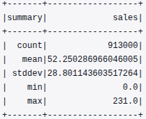
This summary provides a quick overview of the dataset’s numeric distribution:
- The dataset contains 913,000 records, confirming completeness and high data volume.
- The mean sales value is approximately 52.25, with a standard deviation of about 28.80, indicating moderate variability in store-item performance.
- The minimum and maximum sales values (0.0 to 231.0) reflect a realistic range of retail transactions across different store-item combinations.
This descriptive layer establishes the baseline for detecting anomalies, assessing variability, and informing scaling decisions in future modeling phases.
Temporal Sales Trends
To examine monthly sales patterns over time, the year() and month() functions were applied to the date column, followed by a group-wise aggregation of total monthly sales:
from pyspark.sql.functions import year, month, sum as _sum
df = df.withColumn("year", year(col("date"))).withColumn("month", month(col("date")))
monthly_sales = df.groupBy("year", "month").agg(_sum("sales").alias("total_sales")).orderBy("year", "month")
monthly_sales.show(10)
The following output segment illustrates total monthly sales for 2013:
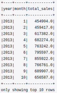
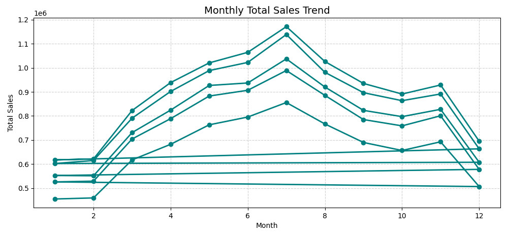
From this, we can infer:
- Steady growth in total sales from January through July.
- A seasonal plateau during mid-year, suggesting cyclical consumer behaviour.
- The presence of temporal variability, which supports the eventual inclusion of time-based features (month, quarter, season) during feature engineering.
This monthly aggregation validates that the pipeline can efficiently summarise time-series data at scale.
Store-Level Performance Analysis
Next, store-level performance was assessed by calculating the average sales per store:
store_avg = df.groupBy("store").agg(avg("sales").alias("avg_sales")).orderBy(col("avg_sales").desc())
store_avg.show(10)
The output revealed clear differences in performance across retail locations:

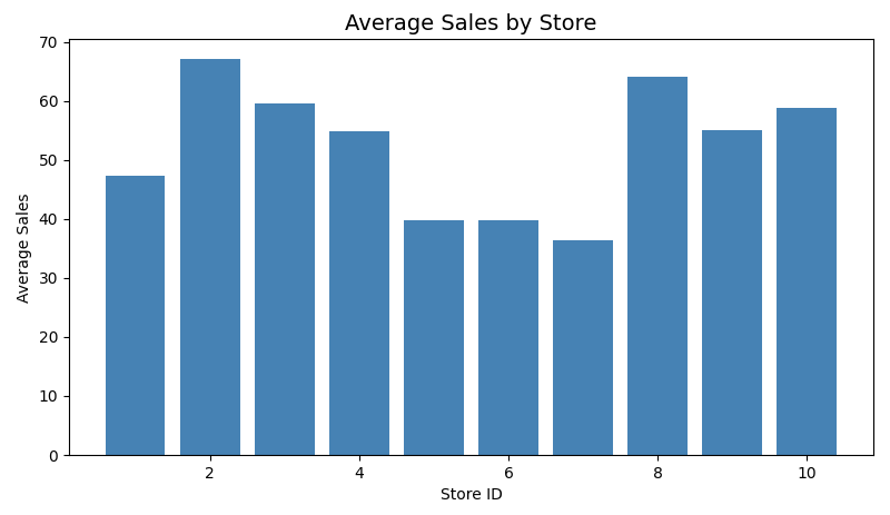
This ranking highlights that Store 2 consistently achieved the highest average sales, while Stores 6 and 7 recorded lower averages. Such store-level variation can be used to build location-specific demand forecasting models or to identify under-performing outlets requiring operational adjustments.
Item-Level Performance Analysis
Similarly, item-level aggregation was performed to identify the top-selling products across all stores:
item_sales = df.groupBy("item").agg(_sum("sales").alias("total_sales")).orderBy(col("total_sales").desc())
item_sales.show(10)
The output was as follows:
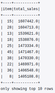
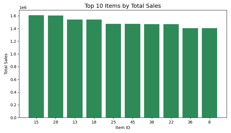
The results show that items 15, 28, and 13 were the highest contributors to total sales during the analyzed period. This insight will be particularly valuable during feature engineering. Item-level popularity can enrich predictive features. Historical demand strength can also be used for machine learning.
Missing Value Check
A missing value check was also performed to confirm the completeness of the dataset:
missing_info = {c: df.filter(col(c).isNull()).count() for c in df.columns}
print(missing_info)
The output retrieved from CloudWatch logs was:
Missing Values Summary:
{'date': 0, 'store': 0, 'item': 0, 'sales': 0, 'sales_scaled_value': 0, 'year': 0, 'month': 0, 'dayofweek': 0}
This confirms that all eight columns are 100 % complete, with no missing or null records. The earlier data-cleaning and imputation steps in the preprocessing stage successfully ensured dataset integrity and consistency. A null-free dataset is essential for distributed computation within Spark. It prevents skewed aggregations and invalid type operations during model training.
Correlation Analysis and Output Persistence
After verifying dataset completeness, a quantitative correlation analysis was performed to understand how key variables interact and influence sales outcomes. This step helps determine which attributes carry predictive potential. It also identifies which attributes may be redundant or weakly associated with the target variable.
Numerical Correlation Analysis
To compute Pearson correlation coefficients between major numeric columns, the following PySpark commands were executed:
# Correlation between key numerical variables
corr_store_item = df.stat.corr("store", "item")
corr_store_sales = df.stat.corr("store", "sales")
corr_item_sales = df.stat.corr("item", "sales")

print("Correlation between store and item:", corr_store_item)
print("Correlation between store and sales:", corr_store_sales)
print("Correlation between item and sales:", corr_item_sales)
The CloudWatch log output was as follows:
Correlation between store and item: 7.063209925969646e-16
Correlation between store and sales: -0.008170361306182861
Correlation between item and sales: -0.05599807493660445
These values provide meaningful insights:
- Store vs Item (≈ 0) — negligible correlation, confirming that store identifiers and item identifiers are independent categorical features.
- Store vs Sales (≈ -0.008) — near-zero correlation, implying that sales variation is not strongly tied to store ID alone. It likely depends more on other temporal or product-specific factors.
- Item vs Sales (≈ -0.056) — weak negative correlation, suggesting minor variation in item-level demand but no strong linear dependency.
These results strengthen the idea that sales behaviour is multi-factorial. It is influenced by time, item, and location combinations. Single attributes alone do not determine it in isolation. This finding directly motivates the feature-engineering phase. In this phase, interaction features and lagged sales trends will be incorporated. This incorporation will help capture these complex relationships.
Inference
By completing correlation computation and persisting the analytical outputs to Amazon S3, the EDA phase achieves full reproducibility and observability.
The dataset is now:
- Fully validated with zero missing values.
- Statistically summarized across temporal, store, and item dimensions.
- Correlated and contextualized, providing actionable insight into feature relationships.
- Persisted in cloud storage, making it readily accessible for model training.
Code Repository
The complete AWS Glue EDA script, glue_script_eda.py, is available in the project’s GitHub repository. This script extends the ETL workflow covered in the previous article. It performs statistical analysis directly within AWS Glue. It also conducts temporal aggregation and computes correlation.
GitHub link: Glue Job Script (EDA)
Conclusion
This initial stage of Exploratory Data Analysis (EDA) is complete. It has successfully laid the groundwork for further development of our demand forecasting model. We have:
- Fully validated the dataset with zero missing values.
- Conducted a statistical summary across temporal, store, and item dimensions.
- Performed a correlation analysis, contextualizing the relationships between key features, providing actionable insights.
- Persisted our findings in cloud storage, ensuring accessibility for subsequent model training.
As we move forward, the next crucial stage will be Feature Engineering and Model Training Preparation. In this phase, we will generate temporal features. We will also create categorical and interaction-based features. These features will enrich our predictive demand forecasting model. This enrichment will allow for more accurate and robust forecasts.


5 Comments